Are you trying to grasp the concept of the Central Limit Theorem? Don’t fret; we’ve got you covered! In this blog post, we will break down the Central Limit Theorem into bite-sized pieces. Moreover, we’ll illustrate this concept with some easy-to-follow R code examples. So, let’s jump right in!

What is the Central Limit Theorem?

The Central Limit Theorem (CLT) is a fundamental statistical concept that explains how the distribution of sample means approaches a normal distribution, regardless of the population’s distribution, provided the sample size is large enough. It allows us to make accurate predictions about a population based on sample data.

Breaking it down

To simplify the Central Limit Theorem further, imagine you are measuring the heights of a group of people. If you take multiple samples of a certain size from this group and calculate the average height of each sample, the distribution of these averages would be approximately normal. This theory holds, especially as the sample size increases.

Now, let’s delve deeper into some hands-on examples using R code.

Getting Started with R

Before we start, make sure to install and load the necessary R packages:

library(tidyverse) #includes dplyr and ggplot2

Example 1: Illustrating the Central Limit Theorem with a Uniform Distribution

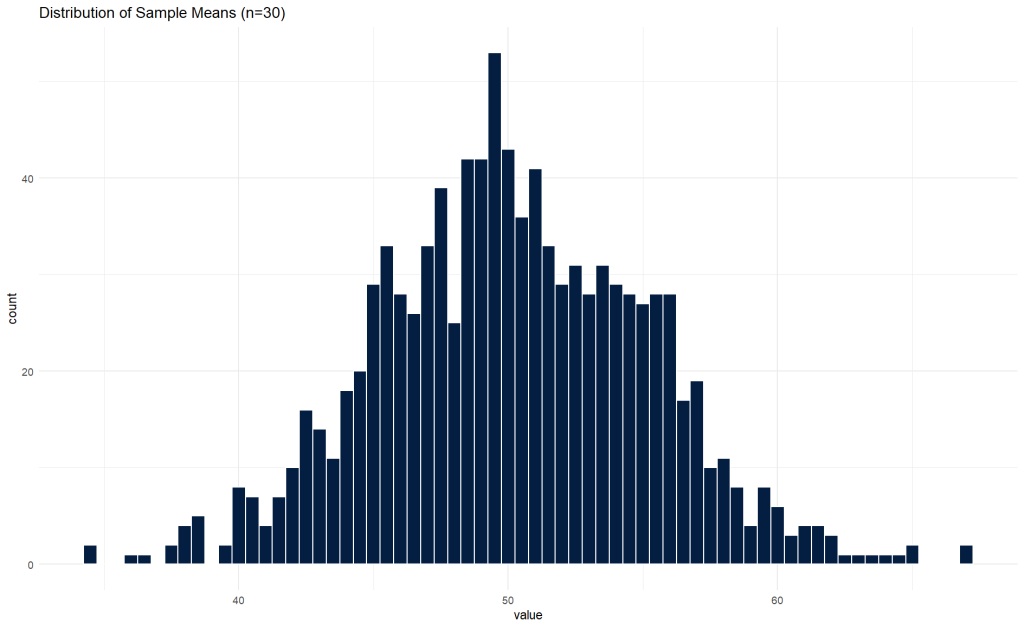
In this example, we will generate a population with a uniform distribution and then demonstrate how the distribution of sample means approaches a normal distribution.

# Setting the seed for reproducibility
set.seed(1701)

# Generating a population with a uniform distribution
population <- runif(100000, min = 0, max = 100)

# Taking multiple samples and calculating the means
sample_means <- replicate(1000, mean(sample(size = 30, x = population))) %>%
  as_tibble()


# Plotting the distribution of sample means
sample_means %>%
  ggplot(aes(x = value)) +
    geom_histogram(binwidth = 0.5, color = "white", fill = '#041e42') +
    ggtitle('Distribution of Sample Means (n=30)') +
    theme_minimal()

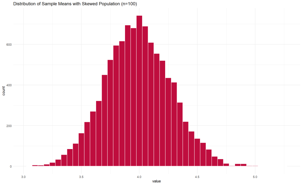
Example 2: Central Limit Theorem with a Skewed Distribution

In this scenario, we will create a population with a skewed distribution and illustrate how the Central Limit Theorem works.

# Generating a population with a skewed distribution
population_skewed <- rgamma(100000, shape = 2, scale = 2)

# Taking multiple samples and calculating the means with a larger sample size
sample_means_skewed <- replicate(10000, mean(sample(size = 100, x = population_skewed))) %>%
  as_tibble()


# Plotting the distribution of sample means
sample_means_skewed %>%
  ggplot(aes(x = value)) +
    geom_histogram(binwidth = 0.05, color = "white", fill = '#bf0d3e') +
    ggtitle('Distribution of Sample Means with Skewed Population (n=100)') +
    theme_minimal()

Implications of the Central Limit Theorem

The Central Limit Theorem holds a prominent place in the field of statistics, essentially forming the backbone of many statistical procedures and theories. Its implications are vast and far-reaching, affecting various disciplines, including economics, psychology, medicine, and even astronomy.

First and foremost, the CLT provides a foundation for making inferences about a population based on sample data. Collecting data from an entire population is often not feasible in real-world scenarios. The CLT, however, allows us to estimate population parameters, such as the mean and standard deviation, from sample statistics with a known degree of uncertainty. This is immensely valuable in medical research where trials are conducted on a sample group before conclusions about the wider population are drawn.

Moreover, the theorem justifies using the normal distribution in many statistical methods, including hypothesis testing and constructing confidence intervals. Even if the population distribution is not normal, the sampling distribution of the sample mean will tend to be normally distributed if the sample size is sufficiently large. This forms the theoretical basis for normality assumption in various statistical modeling techniques, facilitating more straightforward analyses.

Furthermore, the CLT also has implications for quality control and process improvement. In business environments, it is utilized to understand and control process variations, assisting organizations in enhancing their service quality and efficiency. By understanding the properties of distributions of sample means, businesses can set appropriate benchmarks and control limits to monitor their processes effectively.

Lastly, the CLT serves as a tool for risk management in financial sectors. Financial analysts often rely on it to model various scenarios and predict investment outcomes. It enables them to evaluate different investment strategies’ risk and return profiles, helping formulate more informed and rational decisions.

The implications of the CLT are multifaceted, permeating through diverse sectors and facilitating informed decision-making based on sample data. Its influence in shaping modern statistical thinking and methodology cannot be understated, making it an indispensable tool for statisticians, researchers, and data analysts.

Summing Up

As you can see from the R code examples, regardless of the initial population distribution, the distribution of sample means becomes more normal as we increase the sample size, which is the essence of the CLT.

Understanding the Central Limit Theorem is crucial in statistics, helping make predictions and test hypotheses. We hope this blog post has made the CLT more comprehensible, and remember, the larger your sample size, the closer you’ll get to a normal distribution, as stated by the theorem.

Remember to experiment with different sample sizes and populations using R, and witness the Central Limit Theorem in action!