Update: the good people of Reddit pointed out that the sixth ball, the so-called “power ball,” is independent and goes only from 1-25. So that explains the wonky distribution. I’ll have to go back and make some changes. The power of peer review!

Have you ever wondered about the fairness and distribution of the lottery numbers?

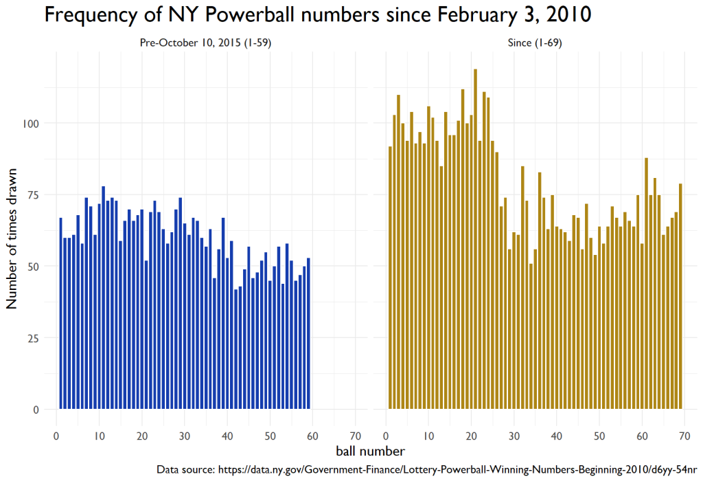
To satisfy this curiosity, I delved into the official Powerball data, readily available from New York’s data portal. An interesting observation was the change in October 2015, where the total number of selectable numbers increased from 59 to 69. This naturally led to the question: are these numbers really evenly distributed both before and after this change?

Let’s unravel the findings.

Did I just solve the lottery?

At first glance, something seemed off. The distribution wasn’t what I initially expected. I mean, this clearly says that I should play 3, 10, 18, 21, 23, and 24.

It wasn’t until a moment of reflection that I remembered a crucial aspect of the Powerball draw: the odds aren’t static—they shift with every single draw.

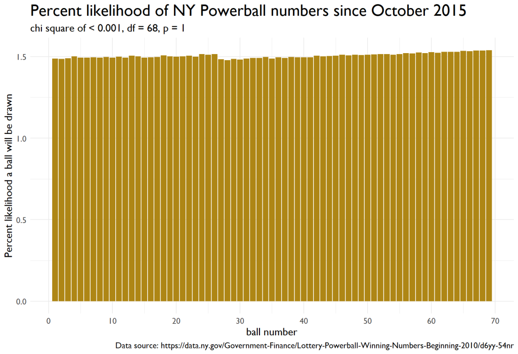
Let’s dive a bit deeper into the post-October 2015 data. When the draw starts, there are 69 balls in the mix, but once a ball is selected, it’s not returned to the pool. This means for the next draw; there are only 68 balls, then 67 for the subsequent one, and so forth. This decreasing pool size affects the probability of any specific ball being chosen as the draw progresses. To truly understand the distribution of winning numbers, it was necessary to compute the likelihood of a ball being selected based on its position in the sequence.

After making these adjustments and computations, I visualized the data. The resulting graph offers a much better look at the Powerball draw.

Conclusion

In wrapping up our analysis of the New York State Powerball data, the results are genuinely intriguing. The dynamic nature of the draw, with changing odds as each ball is picked, adds a layer of complexity to the statistical evaluation. However, by accounting for this mechanism, we’ve painted a more accurate picture of the distribution of winning numbers.

Our deep dive into the post-October 2015 data using the chi-squared test provides a critical insight: while there may be minor variations in the frequency of each number being drawn, the deviations are not statistically significant enough to suggest any inherent bias. In simpler terms, the Powerball draw, from our analysis, appears to be operating as one would expect from a fair game.

It’s always tempting to look for patterns or biases, especially when potential winnings are at stake. However, the beauty of probability is its unpredictability. The Powerball, like many other lotteries, is designed to be random, and our analysis reinforces this nature of the game. So, the next time you pick your numbers, remember that every draw is a fresh start, with every ball having an almost equal chance.

Here’s to hoping luck is on your side!

R Code

library(data.table)
library(tidyverse)
library(extrafont)

df <- fread("C:\\Users\\jonat\\Downloads\\Lottery_Powerball_Winning_Numbers__Beginning_2010.csv") %>% as_tibble()

df1 <- df %>%
  rename("date" = 1,
         "numbers" = 2,
         "multiplier" = 3) %>%
  separate(numbers, into = c("first", "second", "third", "fourth", "fifth", "sixth"), sep = " ") %>%
  mutate(date= lubridate::mdy(date)) %>%
  mutate_if(is.character, as.integer) %>%
  mutate(year = lubridate::year(date))

df2 <- df1 %>%
  pivot_longer(first:sixth, names_to = "sequence", values_to = "number") %>%
  mutate(range = case_when(date < "2015-10-10" ~ "Pre-October 10, 2015 (1-59)",
                           TRUE ~ "Since (1-69)")) %>%
  group_by(range) %>%
  count(number) 

# making the plot
df2 %>%  
  ggplot(aes(x=number, y = n, fill = range)) +
    geom_col(color = "white") +
    theme_minimal() +
    theme(text=element_text(size = 14, family="Gill Sans MT")) +
    scale_x_continuous(breaks = seq(0, 70, by = 10)) +
    facet_wrap(~range) +
    scale_fill_manual(values = c("#153DAE", "#AE8615")) +
    labs(title = "Frequency of NY Powerball numbers since February 3, 2010",
       y = "Number of times ball has been drawn",
       x = "ball number",
       caption = "Data source: https://data.ny.gov/Government-Finance/Lottery-Powerball-Winning-Numbers-Beginning-2010/d6yy-54nr") +
    theme(legend.position = "none") +
    theme(plot.title = element_text(size=22))

observed_freq <- df2$n
total_observed <- sum(observed_freq)
num_numbers <- length(observed_freq)


expected_prob <- rep(1 / num_numbers, num_numbers)


chi_squared_result <- chisq.test(observed_freq, p = expected_prob)


print(chi_squared_result)

best_numbers <- df2 %>%
  ungroup() %>%
  top_n(6, n)

print(best_numbers)

########################
### working off the the sequence

df_sequence <- df1 %>%
  pivot_longer(first:sixth, names_to = "sequence", values_to = "number") %>%
  mutate(range = case_when(date < "2015-10-10" ~ "Pre-October 10, 2015 (1-59)",
                           TRUE ~ "Since (1-69)")) %>%
  filter(grepl("Since", range))

sequence_lookup <- tibble(
  sequence = c("first", "second", "third", "fourth", "fifth", "sixth"),
  balls_left = 69:64
)

# Join the sequence lookup to the data and compute likelihood
df5 <- df_sequence %>%
  left_join(sequence_lookup, by = "sequence") %>%
  group_by(number) %>%
  summarise(likelihood = sum(1 / balls_left) / n()) %>%
  mutate(percentage_likelihood = likelihood * 100)

df5 %>%
  ggplot(aes(x=number, y = percentage_likelihood)) +
    geom_col(fill = "#AE8615") +
    theme_minimal() +
    theme(text=element_text(size = 14, family="Gill Sans MT")) +
    scale_x_continuous(breaks = seq(0, 70, by = 10)) +
    #scale_fill_manual(values = c("#153DAE", "#AE8615")) +
    labs(title = "Percent likelihood of NY Powerball numbers since October 2015",
         subtitle = "chi square of < 0.001, df = 68, p = 1",
         y = "Percent likelihood a ball will be drawn",
         x = "ball number",
         caption = "Data source: https://data.ny.gov/Government-Finance/Lottery-Powerball-Winning-Numbers-Beginning-2010/d6yy-54nr") +
    theme(legend.position = "none") +
    theme(plot.title = element_text(size=22))

# Compute the observed counts from likelihood
observed_counts <- df5$likelihood * total_picks

# Expected counts for each ball if evenly distributed
expected_counts <- rep(total_picks / 69, times=nrow(result))

test_result <- chisq.test(observed_counts, p = expected_counts/sum(expected_counts))

print(test_result)